Single-Source Shortest Path：Dijkstra's Algorithm

先備知識與注意事項

本篇文章將介紹另一種處理Single-Source Shortest Path的方法：Dijkstra's Algorithm。
演算法的概念依然需要：

Relaxation
Convergence property
Path-relaxation property

在演算法中，將會使用到Min-Priority Queue，包含三個基本操作(operation)：

ExtractMin()
DecreaseKey()
MinHeapInsert()，不過本文以BuildMinHeap()取代；

若讀者需要稍作複習，請參考：

Dijkstra's Algorithm

若某一directed graph中，所有edge的weight皆為非負實數(\(weight\geq 0\))，如圖一(a)，便能夠使用Dijkstra's Algorithm處理這個directed graph上的Single-Source Shortest Path問題。

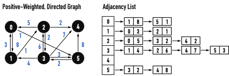
圖一(a)。

Dijkstra's Algorithm是一種「每次挑選當前最佳選擇(optimal solution)」的Greedy Algorithm：

把vertex分成兩個集合，其中一個集合「S」中的vertex屬於「已經找到從起點vertex出發至該vertex的最短路徑」，另一個集合「Q」中的vertex則還沒有。
- 非常重要：這裡的Q就是Min-Priority Queue，其中每一個HeapNode的element即為「vertex的index」，key即為「vertex的distance」，表示從起點走到該vertex的path成本。
對所有vertex的predecessor與distance進行初始化(見圖一(b))，並更新起點vertex之distance為\(0\)；
若Graph中有\(V\)個vertex，便執行\(V\)次迴圈。
在每一個迴圈的開始，從Q中挑選出「distance值最小」的vertex，表示已經找到「從起點vertex抵達該vertex之最短距離」，並將該vertex從Q中移除，放進S集合。
- 利用ExtractMin()挑選「distance值最小」的vertex，即為Greedy Algorithm概念。
每一次迴圈都會藉由Relax()更新「從起點vertex到達仍屬於Q集合的vertex之path距離」，並將path距離存放於distance[]。並且利用DecreaseKey()更新Q中vertex的Key(也就是distance)。
步驟四與步驟五為完整的一次迴圈。
進到下一個迴圈時，會繼續從Q中挑選出「distance最小」的vertex，放進S。
重複上述步驟，直到Q中的vertex都被放進S為止。

如此便能得到從起點vertex抵達其餘vertex的最短路徑。

演算法將使用兩項資料項目predecessor[]與distance[]，其功能如下：

predecessor[]：記錄vertex是被哪個vertex所找到，由predecessor[]可以還原出Predecessor Subgraph，也就是Shortest-Path Tree。
distance[]：記錄從起點vertex走到特定vertex的path之weight總和。

以下以圖一(a)之Graph為例，以vertex(0)為起點，進行Dijkstra's Algorithm。

首先，對predecessor[]和distance[]進行初始化：

所有vertex的predecessor[]先設為\(-1\)。
- 若到演算法結束時，vertex(X)之predecessor[X]仍等於\(-1\)，表示從起點vertex走不到vertex(X)。
所有vertex的distance[]先設為「無限大(\(\infty\))」。
- 若在演算法結束時，distance[]仍為「無限大(\(\infty\))」，表示，從起點vertex走不到vertex(X)。
把起點vertex(0)之distance[0]設為\(0\)，如此一來，當挑選Min-Priority Queue中，distance[]值最小的vertex，進行路徑探索時，就會從vertex(0)開始。

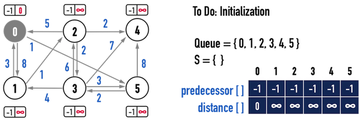
圖一(b)。

接著便進入演算法的主要迴圈，包含兩個步驟：

ExtractMin()：從Min-Priority Queue，也就是Q中，選出distance最小的vertex，並將其從Q中移除。
Relax()以及DecreaseKey()：對選出的vertex所連結的edge進行Relax()，更新distance與predecessor，並同步更新Q。

第一次迴圈：

從Q中以ExtractMin()，取得目前distance值最小的vertex：起點vertex(0)。
建立一個變數int u記住vertex(0)，並將vertex(0)從Q移除，表示已經找到從起點vertex走到vertex(0)的最短路徑，見圖二(a)。

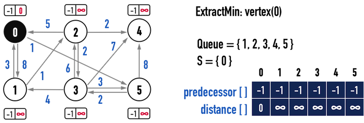
圖二(a)。

接著，以vertex(0)為探索起點，尋找所有「從vertex(0)指出去」的edge，進行：

Relax()：以圖二(b)為例，從vertex(0)能夠走到vertex(1)、vertex(5)，便利用Relax()更新從起點vertex，經過vertex(0)後抵達vertex(1)、vertex(5)的path之weight總和，存放進distance[]，同時更新predecessor[]。
- vertex(1)能夠從vertex(0)以成本「\(8\)」走到，比原先的「無限大(\(\infty\))」成本要低，因此，更新：
  - distance[1]=distance[0]+weight(0,1)；
  - predecessor[1]=0。
- 對vertex(5)比照辦理。
DecreaseKey()：在更新distance[]之後，也要同步更新Q中HeapNode的資料。

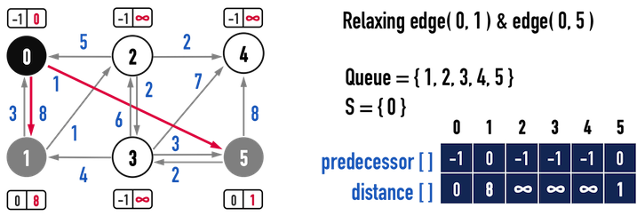
圖二(b)。

第二次迴圈：

繼續從Q中選出distance最小的vertex(5)，並將vertex(5)從Q中移除，表示已經找到「從起點vertex(0)走到vertex(5)」的最短距離，如圖三(a)。

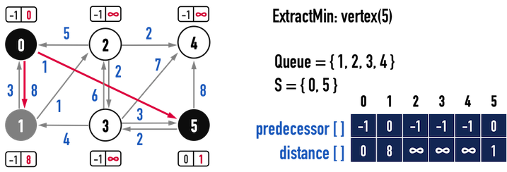
圖三(a)。

關鍵是，為什麼從Q中挑選distance最小的vertex(X)，就能肯定已經找到「從起點vertex走到vertex(X)之最短路徑」，distance[X]\(=\delta(0,X)\)？

這裡不進行嚴謹證明(證明請參考：Ashley Montanaro：Priority queues and Dijkstra’s algorithm)，只就基本條件推論。

前面提到，Dijkstra's Algorithm的使用時機是，當Graph中的weight皆為非負實數(\(weight\geq 0\))，此時：

Graph中的所有cycle之wieght總和必定是正值(positive value)；
亦即，路徑中的edge越多，其weight總和只會增加或持平，不可能減少。

那麼再看圖三(a)，從vertex(0)走到vertex(5)有兩個選擇：

一個是經過edge(0,5)，成本為\(1\)；
另一個是經過edge(0,1)，再經過其他vertex(例如，\(Path:0-1-2-3-5\))，最後抵達vertex(5)，由於edge(0,1)之weight已經是\(8\)，可以確定的是，經過edge(0,1)的這條path之weight總和必定大於\(8\)。

顯然，直接經過edge(0,5)會是從vertex(0)走到vertex(5)最短的路徑。

更廣義地說，從Q中挑選distance最小之vertex，並將其從Q中移除，必定表示，已經找到從起點vertex走到該vertex之最短路徑。

接著，重複上述步驟：

Relax()：對所有「從vertex(5)指出去」的edge進行Relaxation。
DecreaseKey()：同步更新Q中的vertex之distance[]。

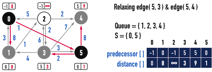
圖三(b)。

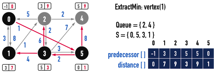
接下來，第三次迴圈至第六次迴圈(直到Q中的vertex都被移除)的步驟如上述，見圖四(a)-圖七(a)。

第三次迴圈：

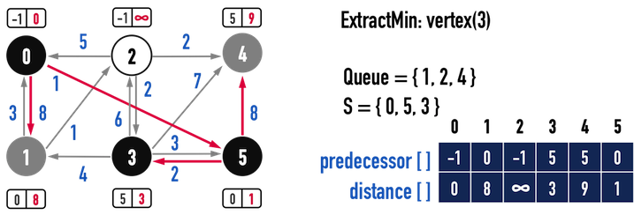
圖四(a)。

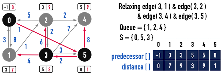
圖四(b)。

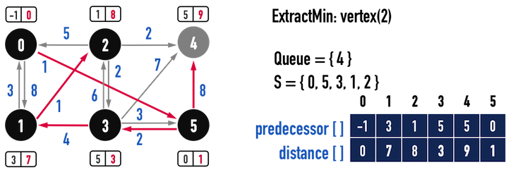
第四次迴圈：

圖五(a)。

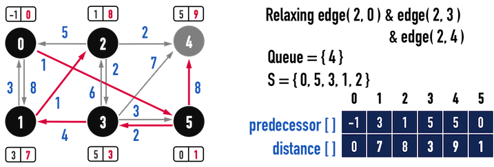
圖五(b)。

第五次迴圈：

圖六(a)。

圖六(b)。

第六次迴圈：

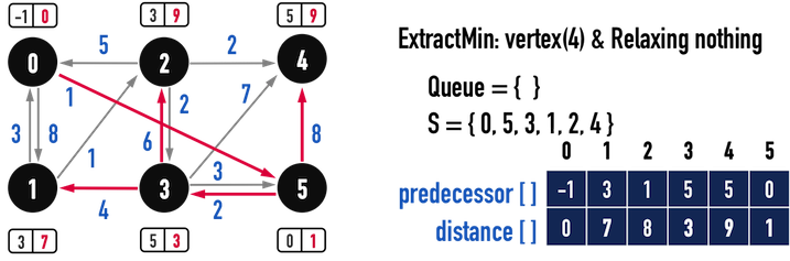
圖七(a)。

圖七(a)便是從vertex(0)走到Graph中其餘vertex之最短路徑Predecessor Subgraph。

程式碼

程式碼包含幾個部分：

class BinaryHeap與struct HeapNode：以Binary Heap實現Min-Priority Queue，概念與範例程式碼請參考Priority Queue：Binary Heap。

class Graph_SP：

基本的資料項目：AdjList、num_vertex、predecessor、distance。
Relax()、InitializeSingleSource()之功能與Bellman-Ford Algorithm所使用相同。
Dijkstra()：功能如前一小節所述。
把class BinaryHeap設為class Graph_SP的「friend」，才能夠把distance[]放進Min Heap中。

以及main()：建立如圖一(a)之AdjList，並進行Dijkstra()。

// C++ code
#include <iostream>
#include <vector>
#include <list>
#include <utility>          // for std::pair<>
#include <iomanip>          // for std::setw()
#include <cmath>            // for std::floor
#include "Priority_Queue_BinaryHeap.h"

const int Max_Distance = 100;
class Graph_SP{             // SP serves as Shortest Path
private:
    int num_vertex;
    std::vector<std::list<std::pair<int,int>>> AdjList;
    std::vector<int> predecessor, distance;
    std::vector<bool> visited;
public:
    Graph_SP():num_vertex(0){};
    Graph_SP(int n):num_vertex(n){
        AdjList.resize(num_vertex);
    }
    void AddEdge(int from, int to, int weight);
    void PrintDataArray(std::vector<int> array);
    void PrintIntArray(int *array);

    void InitializeSingleSource(int Start);     // 以Start作為起點
    void Relax(int X, int Y, int weight);       // edge方向：from X to Y

    void Dijkstra(int Start = 0);        // 需要Min-Priority Queue
    friend class BinaryHeap;             // 以Binary Heap實現Min-Priority Queue
};
void Graph_SP::Dijkstra(int Start){

    InitializeSingleSource(Start);

    BinaryHeap minQueue(num_vertex);   // object of min queue
    minQueue.BuildMinHeap(distance);

    visited.resize(num_vertex, false);   // initializa visited[] as {0,0,0,...,0}

    while (!minQueue.IsHeapEmpty()) {
        int u = minQueue.ExtractMin();
        for (std::list<std::pair<int, int>>::iterator itr = AdjList[u].begin();
             itr != AdjList[u].end(); itr++) {

            Relax(u, (*itr).first, (*itr).second);
            minQueue.DecreaseKey((*itr).first, distance[(*itr).first]);
        }
    }
    std::cout << "\nprint predecessor:\n";
    PrintDataArray(predecessor);
    std::cout << "\nprint distance:\n";
    PrintDataArray(distance);
}
void Graph_SP::InitializeSingleSource(int Start){

    distance.resize(num_vertex);
    predecessor.resize(num_vertex);

    for (int i = 0; i < num_vertex; i++) {
        distance[i] = Max_Distance;
        predecessor[i] = -1;
    }
    distance[Start] = 0;
}
void Graph_SP::Relax(int from, int to, int weight){

    if (distance[to] > distance[from] + weight) {
        distance[to] = distance[from] + weight;
        predecessor[to] = from;
    }
}
void Graph_SP::AddEdge(int from, int to, int weight){

    AdjList[from].push_back(std::make_pair(to,weight));
}
void Graph_SP::PrintDataArray(std::vector<int> array){
    for (int i = 0; i < num_vertex; i++)
        std::cout << std::setw(4) << i;
    std::cout << std::endl;
    for (int i = 0; i < num_vertex; i++)
        std::cout << std::setw(4) << array[i];
    std::cout << std::endl;
}
int main(){

    Graph_SP g9(6);
    g9.AddEdge(0, 1, 8);g9.AddEdge(0, 5, 1);
    g9.AddEdge(1, 0, 3);g9.AddEdge(1, 2, 1);
    g9.AddEdge(2, 0, 5);g9.AddEdge(2, 3, 2);g9.AddEdge(2, 4, 2);
    g9.AddEdge(3, 1, 4);g9.AddEdge(3, 2, 6);g9.AddEdge(3, 4, 7);g9.AddEdge(3, 5, 3);
    g9.AddEdge(5, 3, 2);g9.AddEdge(5, 4, 8);

    g9.Dijkstra(0);

    return 0;
}

output:

new key is larger than current key
new key is larger than current key

print predecessor:
   0   1   2   3   4   5
  -1   3   1   5   5   0

print distance:
   0   1   2   3   4   5
   0   7   8   3   9   1

小小備註(可能不是很重要)：

output中的「new key is larger than current key」來自於Min-Priority Queue中的DecreaseKey()。
DecreaseKey()只允許將Min-Priority Queue中的node之Key「降低」，不能「增加」，所以當要求「增加」時，便中止該函式。

那麼以此例而言，什麼時候會出現「new key is larger than current key」呢？

就是當vertex(X)想要對vertex(Y)進行Relaxation卻失敗的時候，以此例而言：

第一次發生在圖四(a)與圖四(b)，要以vertex(3)對其他「還存在Min-Priority Queue中」而且「與vertex(3)相連」的vertex進行Relaxation時(在vertex(3)因為distance最小而被當作起點之前，vertex(0)與vertex(5)已經從Q中移除了，因此目前只剩下vertex(1)、vertex(2)、vertex(4)與之相連)，因為vertex(4)當下的distance(從vertex(5)走到vertex(4)的成本)會比從vertex(3)走到vertex(4)還低(成本distance[3]+weight(3,4)為\(3+7=10\))，所以在Relaxation後，distance[4]維持不變，那麼在minQueue進行DecreaseKey()時，就不會對vertex(4)的Key(也就是distance[4])進行調整。
第二次發生在圖六(a)與圖六(b)，以vertex(2)對vertex(4)進行Relaxation時，理由與第一次一樣：「從vertex(2)走到vertex(4)的成本」比「從vertex(5)走到vertex(4)的成本」還高，所以不更新distance[4]。

最後，關於Dijkstra's Algorithm之時間複雜度，會因為Min-Priority Queue所使用的資料結構(例如，Binary Heap或是Fibonacci Heap)而有所差異，可能最差從\(O(V^2+E)\)到最好\(O(V\log V+E)\)，請參考以下連結之討論：

以上便是Dijkstra's Algorithm之介紹。

讀者不妨嘗試比較Dijkstra's Algorithm與Bellman-Ford Algorithm之差異，一般情況下，Dijkstra's Algorithm應該會較有效率，不過限制是Graph之weight必須是非負實數(nonnegative real number)，若遇到weight為負數時，仍需使用Bellman-Ford Algorithm。

參考資料：

Shortest Path系列文章

Shortest Path：Intro(簡介)
Single-Source Shortest Path：Bellman-Ford Algorithm
Single-Source Shortest Path：on DAG(directed acyclic graph)
Single-Source Shortest Path：Dijkstra's Algorithm
All-Pairs Shortest Path：Floyd-Warshall Algorithm

回到目錄：

目錄：演算法與資料結構