先備知識與注意事項
本篇文章將介紹Bellman-Ford Algorithm來回應上一篇Single-Source Shortest Path:Intro(簡介)的問題,演算法的概念主要圍繞在:
- Relaxation
- Convergence property
- Path-relaxation property
建議讀者可以先進傳送門精彩回顧一下。
目錄
Graph之表示法(representation)
在BFS/DFS系列文章使用Adjacency List代表Graph,不過edge上沒有weight,可以使用如下資料結構:
std::vector<std::list<int>> AdjList;
MST系列文章的Graph利用Adjacency Matrix,因此可以使用如下資料結構,把weight放進矩陣之元素:
std::vector<std::vector<int>> AdjMatrix;
本篇文章將利用Adjacency List來代表weighted edge,方法是使用C++標準函式庫(STL)的std::pair<int,int>,使得AdjList的資料結構更新為:
std::vector<std::list<std::pair<int,int>>> AdjList;
若有一條從vertex(0)(from)指向vertex(1)(to)的edge(0,1)之weight為\(5\),若利用新的AdjList表示,如圖一:
- 將
from以std::vector的index表示; - 每一個
std::pair<int,int>都是一個std::list的node; - 將
to放在std::pair<int,int>的第一個int資料項; - 將weight放在
std::pair<int,int>的第二個int資料項,
關於std::pair<int,int>的用法,可以參考:Cplusplus:std::pair。
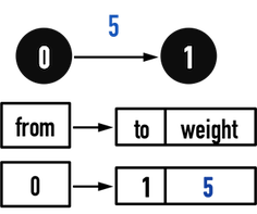
圖一。
Bellman-Ford Algorithm
根據Path-Relaxation Property,考慮一條從vertex(0)到vertex(K)之路徑\(P:v_0-v_1-...-v_K\),如果在對path之edge進行Relax()的順序中,曾經出現edge(v0,v1)、edge(v1,v2)、...、edge(vK-1,vK)的順序,那麼這條path一定是最短路徑,滿足distance[K]\(=\delta(v_0,v_K)\)。
- 在對edge(v1,v2)進行
Relax()之前,只要已經對edge(v0,v1)進行過Relax(),那麼,不管還有其餘哪一條edge已經進行過Relax(),distance[2]必定會等於\(\delta(0,2)\),因為Convergence property。
Bellman-Ford Algorihm就用最直覺的方式滿足Path-Relaxation Property:
- 一共執行\(|V|-1\)次迴圈。
- 在每一次迴圈裡,對「所有的edge」進行
Relax()。 - 經過\(|V|-1\)次的「所有edge之
Relax()」後,必定能夠產生「按照最短路徑上之edge順序的Relax()順序」,也就能夠得到最短路徑。- 由於從起點走到任一vertex之最短路徑,最多只會有\(|V|-1\)條edge,因此,執行\(|V|-1\)次迴圈必定能夠滿足「最壞情況」(worst case)。
考慮如圖二(a)之Graph,以vertex(0)作為起點。
並且根據圖二(a)之Adjacency List,得到在Bellman-Ford Algorihm中對所有edge進行Relax()之順序如圖二(b)。
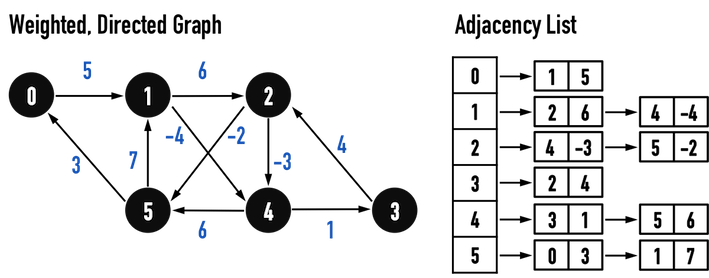
圖二(a)。
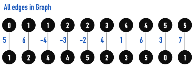
圖二(b):根據圖二(a)之AdjList,對所有edge進行Relax()之順序。
首先,對Graph的資料項目distance與predecessor進行初始化,見圖二(c):
distance:將起點vertex之distance設為\(0\),並將其餘vertex之distance設為無限大(\(\infty\))。- 如果在演算法結束後,某個vertex之
distance仍然無限大(\(\infty\)),則表示Graph中沒有一條path能夠從起點vertex走到該vertex。 - 回顧
Relax(),因為只有起點vertex(0)之distance設為\(0\),其餘distance都是無限大,因此,在進行「所有edge之Relax()」時,一定是從與起點vertex(0)相連之edge先開始。
- 如果在演算法結束後,某個vertex之
predecessor:將所有vertex之predecessor設為\(-1\),表示目前還沒有predecessor。對其餘vertex來說,可以想成還沒有被起點vertex找到。
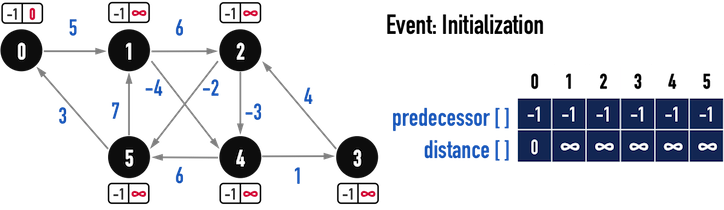
圖二(c)。
接著開始\(|V|-1\)次的迴圈,並在每次迴圈,都對「所有edge」進行Relax()。
(此例,共\(5\)次迴圈,每次按照圖二(b)之順序處理\(10\)條edge)。
第一次迴圈(iteration#1)
對第一條edge(0,1)進行Relax(),見圖三(a):
- 比較
distance[1]與distance[0]+w(0,1),發現」從vertex(0)走到vertex(1)」之成本較原先的成本低(原先的成本即為distance[1]),因此更新distance[1]為distance[0]+w(0,1)。 - 同時更新
predecessor[1]=0,表示vertex(1)是從vertex(0)走過去的。
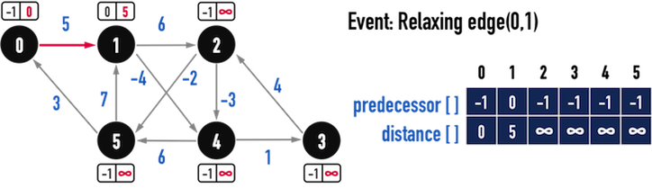
圖三(a)。
對第二、三條edge(1,2)、edge(1,4)進行Relax(),見圖三(b):
- 由於
distance[2]與distance[4]皆大於從vertex(1)走過去的成本,因此更新:distance[2]=distance[1]+w(1,2);distance[4]=distance[1]+w(1,4);
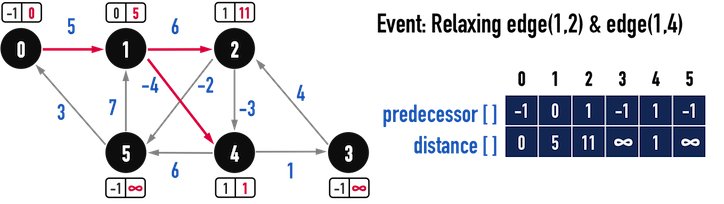
圖三(b)。
對第四、五條edge(2,4)、edge(2,5)進行Relax(),見圖三(c):
- 由於
distance[4]小於「從vertex(2)走過去的成本(distance[2]+w(2,4)),因此,仍維持從vertex(1)走到vertex(4)之路徑。 - 而
distance[5]大於distance[2]+w(2,5),因此更新:distance[5]=distance[2]+w(2,5);predecessor[5]=2;
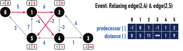
圖三(c)。
對第六條edge(3,2)進行Relax(),見圖三(d):
- 顯然,「從vertex(1)走到vertex(2)」之成本
distance[2]遠小於「從vertex(3)走到vertex(2)」之成本distance[3]+w(2,3),因此,不更新抵達vertex(2)之路徑。
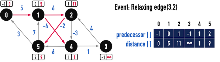
圖三(d)。
對第七、八條edge(4,3)、edge(4,5)進行Relax(),見圖三(e):
- 由於
distance[3]大於從vertex(4)走到vertex(3)的成本(distance[4]+w(4,3)),因此更新:distance[3]=distance[4]+w(4,3);predecessor[3]=4;
- 而且
distance[5]也大於distance[4]+w(4,5),表示「從vertex(4)走到vertex(5)」會比「從vertex(2)走到vertex(5)」還近,便更新:distance[5]=distance[4]+w(4,5);predecessor[5]=4;
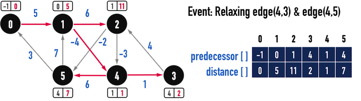
圖三(e)。
對第九、十條edge(5,0)、edge(5,1)進行Relax(),見圖三(f):
- 比較
distance及edge之weight後發現,從vertex(5)走到vertex(0)與vertex(1)之成本皆高於當前走到此二vertex之路徑,因此不更新。
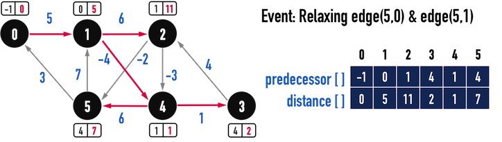
圖三(f)。
經過了第一次迴圈的洗禮,大致能夠掌握Relax()的精髓:如果有比目前的成本更低的路徑,就選擇那條路徑。
例如,圖三(c)中,原本從vertex(0)走到vertex(5)的路徑是\(Path:0-1-2-5\),但是在圖三(e)時,發現了更短的路徑\(Path:0-1-4-5\),便更新其成為目前「從vertex(0)走到vertex(5)」的最短路徑。
還有沒有可能更新出成本更低的路徑?
當然有,因為第一次迴圈的Relax()明顯沒有更新到和edge(3,2)有關路徑,其原因在於,Relax()進行的edge順序。
在第一次迴圈中,是先對edge(3,2)進行Relax(),不過此時的distance[3]還是無限大,因此沒有作用,之後才更新出「從vertex(4)走到vertex(3)」的路徑。
就圖三(f)看來,distance[2]為\(11\),而\(Path:0-1-4-3-2\)之成本只有\(6\),顯然是低於當前的路徑\(Path:0-1-2\)。
因此需要\(|V|-1\)次迴圈,以確保演算法一定能找到最短路徑。
第二次直到第五次迴圈的邏輯同上,在此就不再贅述。
最後得到的最短路徑之Predecessor Subgraph如圖三(g):
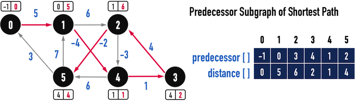
圖三(g)。
根據圖三(g),從vertex(0)走到Graph中其餘vertex之最短路徑為\(Path:0-1-4-3-2-5\),若把Bellman-Ford Algorithm中,每一次迴圈對所有edge進行Relax()之順序攤開,如圖三(h),可以驗證Bellman-Ford Algorithm確實滿足Path-Relaxation Property,按照最短路徑之順序對edge進行Relax()。
(Bellman-Ford Algorithm就是暴力解決,當然會滿足。)
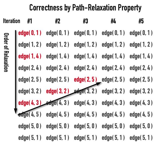
圖三(h)。
程式碼
程式碼包含幾個部分:
class Graph_SP:
- 使用
AdjList,並利用std::pair<int,int>儲存edge的weight。 InitializeSingleSource(int Start):對資料項目distance與predecessor進行初始化,並以int Start作為最短路徑之起點。Relax():對edge進行Relaxation的主要函式。BellmanFord():進行Bellman-Ford Algorithm的主要函式,內容如前一小節所述。
以及main():建立如圖二(a)之AdjList,並進行BellmenFord()。
// C++ code
#include <iostream>
#include <vector>
#include <list>
#include <utility>          // for std::pair<>
#include <iomanip>          // for std::setw()

const int Max_Distance = 100;
class Graph_SP{             // SP serves as Shortest Path
private:
    int num_vertex;
    std::vector<std::list<std::pair<int,int>>> AdjList;
    std::vector<int> predecessor, distance;
public:
    Graph_SP():num_vertex(0){};
    Graph_SP(int n):num_vertex(n){
        AdjList.resize(num_vertex);
    }
    void AddEdge(int from, int to, int weight);
    void PrintDataArray(std::vector<int> array);

    void InitializeSingleSource(int Start);     // 以Start作為起點
    void Relax(int X, int Y, int weight);       // 對edge(X,Y)進行Relax
    bool BellmanFord(int Start = 0);            // 以Start作為起點
                                                // if there is negative cycle, return false
};

bool Graph_SP::BellmanFord(int Start){

    InitializeSingleSource(Start);

    for (int i = 0; i < num_vertex-1; i++) {                // |V-1|次的iteration
        // for each edge belonging to E(G)
        for (int j = 0 ; j < num_vertex; j++) {             // 把AdjList最外層的vector走一遍
            for (std::list<std::pair<int,int> >::iterator itr = AdjList[j].begin();
                 itr != AdjList[j].end(); itr++) {          // 各個vector中, 所有edge走一遍
                Relax(j, (*itr).first, (*itr).second);
            }
        }
    }

    // check if there is negative cycle
    for (int i = 0; i < num_vertex; i++) {
        for (std::list<std::pair<int,int> >::iterator itr = AdjList[i].begin();
             itr != AdjList[i].end(); itr++) {
            if (distance[(*itr).first] > distance[i]+(*itr).second) {   // i是from, *itr是to
                return false;
            }
        }
    }

    // print predecessor[] & distance[]
    std::cout << "predecessor[]:\n";
    PrintDataArray(predecessor);
    std::cout << "distance[]:\n";
    PrintDataArray(distance);

    return true;
}
void Graph_SP::PrintDataArray(std::vector<int> array){
    for (int i = 0; i < num_vertex; i++)
        std::cout << std::setw(4) << i;
    std::cout << std::endl;
    for (int i = 0; i < num_vertex; i++)
        std::cout << std::setw(4) << array[i];
    std::cout << std::endl << std::endl;
}
void Graph_SP::InitializeSingleSource(int Start){

    distance.resize(num_vertex);
    predecessor.resize(num_vertex);

    for (int i = 0; i < num_vertex; i++) {
        distance[i] = Max_Distance;
        predecessor[i] = -1;
    }
    distance[Start] = 0;
}
void Graph_SP::Relax(int from, int to, int weight){

    if (distance[to] > distance[from] + weight) {
        distance[to] = distance[from] + weight;
        predecessor[to] = from;
    }
}
void Graph_SP::AddEdge(int from, int to, int weight){
    AdjList[from].push_back(std::make_pair(to,weight));
}

int main(){

    Graph_SP g7(6);
    g7.AddEdge(0, 1, 5);
    g7.AddEdge(1, 4, -4);g7.AddEdge(1, 2, 6);
    g7.AddEdge(2, 4, -3);g7.AddEdge(2, 5, -2);
    g7.AddEdge(3, 2, 4);
    g7.AddEdge(4, 3, 1);g7.AddEdge(4, 5, 6);
    g7.AddEdge(5, 0, 3);g7.AddEdge(5, 1, 7);

    if (g7.BellmanFord(0))
        std::cout << "There is no negative cycle.\n";
    else
        std::cout << "There is negative cycle.\n";

    return 0;
}
output:
predecessor[]:
   0   1   2   3   4   5
  -1   0   3   4   1   2

distance[]:
   0   1   2   3   4   5
   0   5   6   2   1   4

There is no negative cycle.
檢查Graph中是否存在negative cycle
聰明的讀者一定已經發現了,BellmanFord()還有個功能,可以檢查Graph中是否存在negative cycle。
上一篇文章Single-Source Shortest Path:Intro(簡介)曾經提到,塵世間最痛苦的事情莫過於在處理Single-Source Shortest Path問題時碰上negative cycle,因為negative cycle存在會使得最短路徑出現\(-\infty\)。
若存在從vertex(from)指向vertex(to)的edge(from,to),並具有weight,根據Relax()的運作原則,:
- 若
distance[to]\(>\)distance[from]+weight,便更新distance[to]=distance[from]+weight」。
因此,在對Graph中所有edge進行Relax()後,所有edge(from,to)所連結的兩個vertex之distance必定滿足:
distance[to]\(\leq\)distance[from]+weight
而BellmanFord()的檢查方法,便是在\(|V|-1\)次「對所有edge進行Relax()」後,檢查,若存在任何一條edge(from,to)所連結的兩個vertex之distance關係為:
distance[to]\(>\)distance[from]+weight
就表示存在某一條edge之weight永遠可以讓該edge連結之vertex的distance下降,因此Graph中必定存在negative cycle。
以上便是Bellman-Ford Algorithm之介紹。
只要了解:
- Relaxation
- Convergence property
- Path-relaxation property
之概念,即可掌握Bellman-Ford Algorithm的運作邏輯。
下一篇文章將介紹的是,在DAG(directed acyclic graph)中處理Single-Source Shortest Path之演算法。
參考資料:
- Introduction to Algorithms, Ch24
- Fundamentals of Data Structures in C++, Ch6
- Wikipedia:Shortest path problem
- Cplusplus:std::pair
Shortest Path系列文章
Shortest Path:Intro(簡介)
Single-Source Shortest Path:Bellman-Ford Algorithm
Single-Source Shortest Path:on DAG(directed acyclic graph)
Single-Source Shortest Path:Dijkstra's Algorithm
All-Pairs Shortest Path:Floyd-Warshall Algorithm
回到目錄: